Pandas, Execel, Csv
对Pandas基本数据结构、重要方法的介绍,此外还介绍了Pandas的Excel、csv相关工具用法
注:撰写此笔记时,pandas的stable版本为2.2
pandas介绍
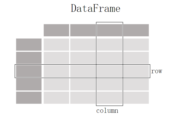
pandas是一个专门处理 表格式(tabular)数据的python工具包,在Pandas中,一个表格式数据被叫做 DataFrame
功能简述
pandas不仅拥有对表格式数据的读写能力,还可以对数据进行绘图、筛选、计算等,本部分对pandas的能力做一个简要的总结,后面再做详细介绍
| 功能 | 描述 |
|---|---|
| 读写数据 | pandas支持多种类型文件的读写(csv, excel, sql, json, parquet…),使用函数read_*进行读取,to_*进行存储 |
| 筛选 | pandas中拥有一些 slicing, selecting, extracting函数,支持数据的分片、选择、提取 |
| 绘图 | pandas也可以对数据进行绘图,得益于Matplotlib库的支持 |
| 插入 | pandas可以通过简单的操作对现有的数据插入新的列/行 |
| 其它 | 数值计算(max, min, mean, counts…),改变表格结构、合并多个文件、处理时间数据、文本数据处理 |
pandas 安装
在anaconda环境下
1
conda install -c <your_forge_name> pandas
使用pip从pypi中安装
1
2
3
4
# 安装 pandas
pip install pandas
# 安装指定的依赖
pip install "pandas[<依赖包名>]"
截至目前pandas要求pip版本最低为19.3
安装正在开发的pandas版本
开发版本通常每天从 anaconda.org 的 PyPI 注册表上传到 Scientific-python-nightly-wheels 索引,可以通过运行来安装它。
1
pip install --pre --extra-index https://pypi.anaconda.org/scientific-python-nightly-wheels/simple pandas
当你想要卸载一个当前pandas时,执行:
1
2
pip uninstall pandas -y
# -y 表示yes,不询问是否确定卸载
依赖
依赖可能会随这版本更新改变,若有不同请参考官网安装教程
必须依赖
| Package | 最低支持版本 |
|---|---|
| NumPy | 1.22.4 |
| python-dateutil | 2.8.2 |
| pytz | 2020.1 |
| tzdata | 2022.7 |
可选依赖
pandas 有许多可选依赖项,仅用于特定方法。例如,pandas.read_hdf()需要pytables包,而DataFrame.to_markdown()需要tabulate包。
当使用了一些方法需要额外的包,若未安装,则会抛出
ImportError
提高性能的依赖(推荐安装)
pip install "pandas[performance]"
| Dependency | Minimum Version | pip extra | Notes |
|---|---|---|---|
| numexpr | 2.8.4 | performance | 通过使用多核以及智能分块和缓存来加速某些数值运算,以实现大幅加速 |
| bottleneck | 1.3.6 | performance | 通过使用专门的 cython 例程来加速某些类型的nan,以实现大幅加速 |
| numba | 0.56.4 | performance | 用于接受 engine="numba" 的操作的替代执行引擎,使用 JIT 编译器,使用 LLVM 编译器将 Python 函数转换为优化的机器代码。 |
可视化依赖
pip install "pandas[plot, output-formatting]"
| Dependency | Minimum Version | pip extra | Notes |
|---|---|---|---|
| matplotlib | 3.6.3 | plot | Plotting library |
| Jinja2 | 3.1.2 | output-formatting | Conditional formatting with DataFrame.style |
| tabulate | 0.9.0 | output-formatting | Printing in Markdown-friendly format (see tabulate) |
数值计算处理依赖
pip install "pandas[computation]"
| Dependency | Minimum Version | pip extra | Notes |
|---|---|---|---|
| SciPy | 1.10.0 | computation | Miscellaneous statistical functions |
| xarray | 2022.12.0 | computation | pandas-like API for N-dimensional data |
Excel依赖
pip install "pandas[excel]"
| Dependency | Minimum Version | pip extra | Notes |
|---|---|---|---|
| xlrd | 2.0.1 | excel | Reading Excel |
| xlsxwriter | 3.0.5 | excel | Writing Excel |
| openpyxl | 3.1.0 | excel | Reading / writing for xlsx files |
| pyxlsb | 1.0.10 | excel | Reading for xlsb files |
| python-calamine | 0.1.7 | excel | Reading for xls/xlsx/xlsb/ods files |
HTML依赖
pip install "pandas[html]"
| Dependency | Minimum Version | pip extra | Notes |
|---|---|---|---|
| BeautifulSoup4 | 4.11.2 | html | HTML parser for read_html |
| html5lib | 1.1 | html | HTML parser for read_html |
| lxml | 4.9.2 | html | HTML parser for read_html |
One of the following combinations of libraries is needed to use the top-level read_html() function:
- BeautifulSoup4 and html5lib
- BeautifulSoup4 and lxml
- BeautifulSoup4 and html5lib and lxml
- Only lxml, although see HTML Table Parsing for reasons as to why you should probably not take this approach.
- if you install BeautifulSoup4 you must install either lxml or html5lib or both.
read_html()will not work with only BeautifulSoup4 installed.- You are highly encouraged to read HTML Table Parsing gotchas. It explains issues surrounding the installation and usage of the above three libraries.
XML依赖
pip install "pandas[xml]"
| Dependency | Minimum Version | pip extra | Notes |
|---|---|---|---|
| lxml | 4.9.2 | xml | XML parser for read_xml and tree builder for to_xml |
SQL数据库依赖
pip install "pandas[postgresql, mysql, sql-other]"
| Dependency | Minimum Version | pip extra | Notes |
|---|---|---|---|
| SQLAlchemy | 2.0.0 | postgresql, mysql, sql-other | SQL support for databases other than sqlite |
| psycopg2 | 2.9.6 | postgresql | PostgreSQL engine for sqlalchemy |
| pymysql | 1.0.2 | mysql | MySQL engine for sqlalchemy |
| adbc-driver-postgresql | 0.8.0 | postgresql | ADBC Driver for PostgreSQL |
| adbc-driver-sqlite | 0.8.0 | sql-other | ADBC Driver for SQLite |
其他类型数据依赖
pip install "pandas[hdf5, parquet, feather, spss, excel]"
| Dependency | Minimum Version | pip extra | Notes |
|---|---|---|---|
| PyTables | 3.8.0 | hdf5 | HDF5-based reading / writing |
| blosc | 1.21.3 | hdf5 | Compression for HDF5; only available on conda |
| zlib | hdf5 | Compression for HDF5 | |
| fastparquet | 2022.12.0 | Parquet reading / writing (pyarrow is default) | |
| pyarrow | 10.0.1 | parquet, feather | Parquet, ORC, and feather reading / writing |
| pyreadstat | 1.2.0 | spss | SPSS files (.sav) reading |
| odfpy | 1.4.1 | excel | Open document format (.odf, .ods, .odt) reading / writing |
从云中访问数据
pip install "pandas[fss, aws, gcp]"
| Dependency | Minimum Version | pip extra | Notes |
|---|---|---|---|
| fsspec | 2022.11.0 | fss, gcp, aws | Handling files aside from simple local and HTTP (required dependency of s3fs, gcsfs). |
| gcsfs | 2022.11.0 | gcp | Google Cloud Storage access |
| pandas-gbq | 0.19.0 | gcp | Google Big Query access |
| s3fs | 2022.11.0 | aws | Amazon S3 access |
剪切板
pip install "pandas[clipboard]".
| Dependency | Minimum Version | pip extra | Notes |
|---|---|---|---|
| PyQt4/PyQt5 | 5.15.9 | clipboard | Clipboard I/O |
| qtpy | 2.3.0 | clipboard | Clipboard I/O |
压缩
pip install "pandas[compression]"
| Dependency | Minimum Version | pip extra | Notes |
|---|---|---|---|
| Zstandard | 0.19.0 | compression | Zstandard compression |
基本数据类型
pandas有两种基本数据类型Series和DataFrame,分别代表一维数据和二维数据
| 维度 | 名字 | 描述 |
|---|---|---|
| 1 | Series | 一维同类型带标签的数组 |
| 2 | DataFrame | 具有潜在异构类型列的通用二维标记、大小可变的表格结构 |
Series
Series 是一个一维标记数组,可以保存任何数据类型(整数、字符串、浮点数、Python 对象等),轴标签统称为索引。
可以理解为Excel表格中的一列,Index就相当于Excel中行编号,只不过这里的Index可以不止为数字
为什么是一列而不是一行呢?因为通常每列数据类型是相同的,Series想表示一组同类型的数据
构造Series
Series 是一个一维标记数组,能够容纳任何数据类型(整数、字符串、浮点数、Python 对象等)。轴标签统称为index。创建 Series 的基本方法是调用:
1
s = pd.Series(data, index=index)
这里的data可以是python的字典、ndarray(n-dimension array,实际上传入的数组必须是1维的)、标量(一个值,比如1),index代表数据轴上的标签,根据data的不同index拥有不同的效果:
当data是字典时
此时可以不传入index,字典对应的key会被对应到每个value的index
1
2
3
4
5
6
7
8
In [7]: d = {"b": 1, "a": 0, "c": 2}

In [8]: pd.Series(d)
Out[8]:
b    1
a    0
c    2
dtype: int64
如果传入了index,如
1
2
3
4
5
6
7
[In 11]: pd.Series(d, index=["b", "c", "d", "a"])
Out[11]:
b    1.0
c    2.0
d    NaN
a    0.0
dtype: float64
NaN(not a number)是在pandas中缺失数据时使用的标准标记
当传入的data是ndarry时
此时index的长度必须与ndarray的长度相同(注:不会像dict那样自动填充NaN),data的index会与传入的index对应,如果不传入index默认值会为[0, ..., len(data)-1]
1
2
3
4
5
6
7
8
9
10
11
12
13
14
15
16
17
18
19
20
21
22
In [3]: s = pd.Series(np.random.randn(5), index=["a", "b", "c", "d", "e"])

In [4]: s
Out[4]:
a    0.469112
b   -0.282863
c   -1.509059
d   -1.135632
e    1.212112
dtype: float64

In [5]: s.index
Out[5]: Index(['a', 'b', 'c', 'd', 'e'], dtype='object')

In [6]: pd.Series(np.random.randn(5))
Out[6]:
0   -0.173215
1    0.119209
2   -1.044236
3   -0.861849
4   -2.104569
dtype: float64
当传入的数据是标量时
此时最好传入index,这个标量的值会被重复到与index的长度一致:
1
2
3
4
5
6
7
8
9
10
11
12
13
14
In [12]: pd.Series(5.0, index=["a", "b", "c", "d", "e"])
Out[12]:
a    5.0
b    5.0
c    5.0
d    5.0
e    5.0
dtype: float64
# 若不传入index
In [12]: pd.Series(5)
In [13]: print(s.array)
out[13]:
0    1
dtype: int64
为什么要用Index?
- 标识和访问数据:索引为数据点提供了一个唯一的标识,这使得可以通过索引标签来访问特定的数据值。没有索引的话,只能使用位置索引(类似于数组的索引)来访问数据。
- 数据对齐:索引使得不同
Series对象之间的数据能够根据索引进行对齐操作。这对于数据运算和合并非常有用。例如,在进行加法运算时,只有索引匹配的数据才会相加。 - 增加数据的描述性:索引标签可以是字符串、日期、时间等,更加直观地描述数据的含义,而不仅仅是数字位置索引。
- 支持时间序列数据:索引尤其在处理时间序列数据时非常有用。时间序列数据的索引通常是时间戳,这使得可以方便地进行时间相关的操作,比如重采样和时间切片。
Series的使用技巧
像数组一样使用(Index无关型操作)
Series拥有iloc属性,它提供通过位置索引(整数索引)的访问和操作Series对象的数据。当只关心数据位置而不是标签时非常有用。
Series.iloc主要有以下几个作用:
- 单个元素访问:可以通过整数索引访问单个元素。
- 切片操作:可以通过整数位置进行切片操作,获取一个子集。
- 布尔索引:可以通过布尔数组进行索引,获取符合条件的子集。
1
2
3
4
5
6
7
8
9
10
11
12
13
14
15
16
17
18
19
20
21
22
23
24
25
26
27
28
# 单个元素访问
import pandas as pd

data = [10, 20, 30, 40, 50]
index = ['a', 'b', 'c', 'd', 'e']
series = pd.Series(data, index=index)

# 访问第二个元素
print(series.iloc[1])  # 输出: 20

# 切片操作
# 获取从第2个到第4个元素(不包括第4个)
print(series.iloc[1:3])

# 输出:
# b    20
# c    30
# dtype: int64

# 使用布尔索引
print(series.iloc[[True, False, True, False, True]])

# 输出:
# a    10
# c    30
# e    50
# dtype: int64
像字典一样使用
Series对象可以通过设置的Index标签像字典一样访问数据
1
2
3
4
5
6
7
8
9
10
11
12
13
14
15
16
17
18
19
20
21
22
23
24
25
In [21]: s["a"]
Out[21]: 0.4691122999071863

In [22]: s["e"] = 12.0

In [23]: s
Out[23]:
a     0.469112
b    -0.282863
c    -1.509059
d    -1.135632
e    12.000000
dtype: float64

In [24]: "e" in s
Out[24]: True

In [25]: "f" in s
Out[25]: False

# 使用get函数
In [27]: s.get("f")

In [28]: s.get("f", np.nan)
Out[28]: nan
向量操作–标签自动对齐
当进行两个向量之间的加法操作时(或其他操作),Series和Numpy array一样不需要使用循环一个一个的计算,可以直接进行操作:
1
2
3
4
5
6
7
8
9
10
11
12
13
14
15
16
17
18
19
20
21
22
23
24
25
26
In [29]: s + s
Out[29]:
a     0.938225
b    -0.565727
c    -3.018117
d    -2.271265
e    24.000000
dtype: float64

In [30]: s * 2
Out[30]:
a     0.938225
b    -0.565727
c    -3.018117
d    -2.271265
e    24.000000
dtype: float64

In [31]: np.exp(s)
Out[31]:
a         1.598575
b         0.753623
c         0.221118
d         0.321219
e    162754.791419
dtype: float64
与Numpy不同的是,Series会根据Index值自动对齐。此外两个Series拥有不同Index也可以进行操作,会自动对其它们重叠的Index,如果一个Index另一个对象没有,则操作结果为 NaN ,最终结果的Index为两个对象Index的并集:
1
2
3
4
5
6
7
8
In [32]: s.iloc[1:] + s.iloc[:-1]
Out[32]:
a         NaN
b   -0.565727
c   -3.018117
d   -2.271265
e         NaN
dtype: float64
name属性
在许多情况下,Series 名称可以自动分配,特别是从 DataFrame 中选择单个列时,该名称将被分配列标签。
DataFrame
DataFrame 是一个二维标记数据结构,其列可能具有不同类型的类型。你可以将它想象成电子表格或 SQL 表,或 Series 对象的字典。它通常是最常用的 pandas 对象。
构造DataFrame
DataFrame可以接收多种输入:
- 一维数组的字典、lists、dicts或
Series(注意复数形式) - 二维数组
- 单个
Series - 另一个
DataFrame - Structured or record ndarray
使用value为Series对象的字典构造
字典中value为Series对象,每个item会被视为一列,列名为item的key,列内容为Series,每个Series都会有Index属性,最终构造出的总Index为所有Index的并集,若某个Series对象无某个index,则会填充NaN
1
2
3
4
5
6
7
8
9
10
11
12
13
14
15
16
17
18
19
20
21
22
23
24
25
26
27
28
In [38]: d = {
   ....:     "one": pd.Series([1.0, 2.0, 3.0], index=["a", "b", "c"]),
   ....:     "two": pd.Series([1.0, 2.0, 3.0, 4.0], index=["a", "b", "c", "d"]),
   ....: }
   ....:
# 直接构造
In [39]: df = pd.DataFrame(d)
In [40]: df
Out[40]:
   one  two
a  1.0  1.0
b  2.0  2.0
c  3.0  3.0
d  NaN  4.0
# 构造时指定Index,则只会保留传入的Index
In [41]: pd.DataFrame(d, index=["d", "b", "a"])
Out[41]:
   one  two
d  NaN  4.0
b  2.0  2.0
a  1.0  1.0
# 构造时传入cloumns参数,则只会保留对应key的item
In [42]: pd.DataFrame(d, index=["d", "b", "a"], columns=["two", "three"])
Out[42]:
   two three
d  4.0   NaN
b  2.0   NaN
a  1.0   NaN
使用value为数组/列表的字典构造
此时所有value对应的数组,长度一定要相同,否则会抛出ValueError。此外如果不传入Index,则Index会使用ange(n)生成,n为长度,如果传入了Index,则要保证传入的Index长度要与数组长度对应,否则也会抛出ValueError
1
2
3
4
5
6
7
8
9
10
11
12
13
14
15
16
17
In [45]: d = {"one": [1.0, 2.0, 3.0, 4.0], "two": [4.0, 3.0, 2.0, 1.0]}
# 不传入Index
In [46]: pd.DataFrame(d)
Out[46]:
   one  two
0  1.0  4.0
1  2.0  3.0
2  3.0  2.0
3  4.0  1.0
# 传入Index
In [47]: pd.DataFrame(d, index=["a", "b", "c", "d"])
Out[47]:
   one  two
a  1.0  4.0
b  2.0  3.0
c  3.0  2.0
d  4.0  1.0
使用dict数组构造
使用
dict构造Series对象时,key被当作了Index,而在此处,key会被当做columns
1
2
3
4
5
6
7
8
9
10
11
12
13
14
15
16
17
18
19
In [53]: data2 = [{"a": 1, "b": 2}, {"a": 5, "b": 10, "c": 20}]

In [54]: pd.DataFrame(data2)
Out[54]:
   a   b     c
0  1   2   NaN
1  5  10  20.0

In [55]: pd.DataFrame(data2, index=["first", "second"])
Out[55]:
        a   b     c
first   1   2   NaN
second  5  10  20.0

In [56]: pd.DataFrame(data2, columns=["a", "b"])
Out[56]:
   a   b
0  1   2
1  5  10
使用tuple字典构造多级列名/行名
可以按照如下方式进行创建一个DataFrame
1
2
3
4
5
6
7
8
9
10
11
12
13
14
15
16
In [57]: pd.DataFrame(
   ....:     {
   ....:         ("a", "b"): {("A", "B"): 1, ("A", "C"): 2},
   ....:         ("a", "a"): {("A", "C"): 3, ("A", "B"): 4},
   ....:         ("a", "c"): {("A", "B"): 5, ("A", "C"): 6},
   ....:         ("b", "a"): {("A", "C"): 7, ("A", "B"): 8},
   ....:         ("b", "b"): {("A", "D"): 9, ("A", "B"): 10},
   ....:     }
   ....: )
   ....:
Out[57]:
       a              b
       b    a    c    a     b
A B  1.0  4.0  5.0  8.0  10.0
  C  2.0  3.0  6.0  7.0   NaN
  D  NaN  NaN  NaN  NaN   9.0
解释:
最外层的key会被解释成列,看前三个item的key分别为(“a”, “b”), (“a”, “a”), (“a”, “c”),它们一级列名都是a,二级列名有三个,依次为b, a, c,因此可以看到输出中,2,3,4列刚好是这样的,同理可以推出b为一级列标题的
内层的key会被解释为Index,它们一级行标题只有”A”,因此输出也只有一个A为一级行标题,二级行标题按照第一次出现的顺序排列
在Excel中,这个数据结构对应如图所示
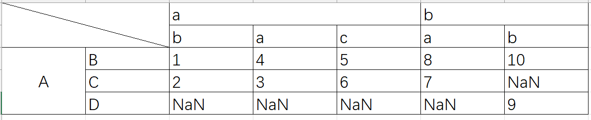
列为 a, b,行为 A, B的值为1,列为 b, b 行为A, B 对应的值为10
使用单个Series创建
因为一个
Series只代表一列,使用单个Series构造的结果也只是一列,并且Series的name属性会被当做列名,Index属性会被保留1 2 3 4 5 6 7 8
In [58]: ser = pd.Series(range(3), index=list("abc"), name="ser") In [59]: pd.DataFrame(ser) Out[59]: ser a 0 b 1 c 2
DataFrame的使用技巧
根据已有的列计算出一个新的列并插入assign()方法链
DataFrame拥有assign()方法,它可以方便地从现有的列派生出一个新的列并插入,它不会改变原来的DataFrame,而是复制一份插入,然后返回
1
2
3
4
5
6
7
8
9
10
11
12
13
14
15
16
17
18
19
In [85]: iris = pd.read_csv("data/iris.data")

In [86]: iris.head()
Out[86]:
   SepalLength  SepalWidth  PetalLength  PetalWidth         Name
0          5.1         3.5          1.4         0.2  Iris-setosa
1          4.9         3.0          1.4         0.2  Iris-setosa
2          4.7         3.2          1.3         0.2  Iris-setosa
3          4.6         3.1          1.5         0.2  Iris-setosa
4          5.0         3.6          1.4         0.2  Iris-setosa

In [87]: iris.assign(sepal_ratio=iris["SepalWidth"] / iris["SepalLength"]).head()
Out[87]:
   SepalLength  SepalWidth  PetalLength  PetalWidth         Name  sepal_ratio
0          5.1         3.5          1.4         0.2  Iris-setosa     0.686275
1          4.9         3.0          1.4         0.2  Iris-setosa     0.612245
2          4.7         3.2          1.3         0.2  Iris-setosa     0.680851
3          4.6         3.1          1.5         0.2  Iris-setosa     0.673913
4          5.0         3.6          1.4         0.2  Iris-setosa     0.720000
也可以传入只有一个参数的函数,这个函数会被用来计算新的列的值
1
2
3
4
5
6
7
8
In [88]: iris.assign(sepal_ratio=lambda x: (x["SepalWidth"] / x["SepalLength"])).head()
Out[88]:
   SepalLength  SepalWidth  PetalLength  PetalWidth         Name  sepal_ratio
0          5.1         3.5          1.4         0.2  Iris-setosa     0.686275
1          4.9         3.0          1.4         0.2  Iris-setosa     0.612245
2          4.7         3.2          1.3         0.2  Iris-setosa     0.680851
3          4.6         3.1          1.5         0.2  Iris-setosa     0.673913
4          5.0         3.6          1.4         0.2  Iris-setosa     0.720000
函数的参数是**kwargs,是一个字典,这个字典的key值会被当做新的列名,value值可以直接是想要插入的值(Series对象或数组),也可以是一个可以调用的对象,会调用此对象计算新的列的值,**kwargs的顺序会被保留,返回值中新的列按照此顺序。
得到某行或某列
| Operation | Syntax | Result |
|---|---|---|
| 选择列 | df[col] | Series |
| 使用label选择行 | df.loc[label] | Series |
| 使用整数进行行定位 | df.iloc[loc] | Series |
| 行切片 | df[5:10] | DataFrame |
| 使用bool向量选择行 | df[bool_vec] | DataFrame |
数据对齐和算术
DataFrame 对象之间的数据对齐会自动在列和索引(行标签)上对齐。同样,生成的对象将具有列标签和行标签的并集。
1
2
3
4
5
6
7
8
9
10
11
12
13
14
15
16
17
18
19
20
21
22
23
24
25
26
27
28
29
30
31
32
33
34
35
36
37
38
39
40
41
42
43
44
45
46
47
48
49
50
51
52
53
54
55
56
57
58
59
60
61
62
63
64
65
66
67
68
69
70
71
72
73
74
75
76
77
78
79
80
81
82
83
84
85
86
87
88
89
90
91
92
93
94
95
96
97
98
99
100
101
102
103
104
105
In [94]: df = pd.DataFrame(np.random.randn(10, 4), columns=["A", "B", "C", "D"])

In [95]: df2 = pd.DataFrame(np.random.randn(7, 3), columns=["A", "B", "C"])

In [96]: df + df2
Out[96]:
          A         B         C   D
0  0.045691 -0.014138  1.380871 NaN
1 -0.955398 -1.501007  0.037181 NaN
2 -0.662690  1.534833 -0.859691 NaN
3 -2.452949  1.237274 -0.133712 NaN
4  1.414490  1.951676 -2.320422 NaN
5 -0.494922 -1.649727 -1.084601 NaN
6 -1.047551 -0.748572 -0.805479 NaN
7       NaN       NaN       NaN NaN
8       NaN       NaN       NaN NaN
9       NaN       NaN       NaN NaN

In [97]: df - df.iloc[0]
Out[97]:
          A         B         C         D
0  0.000000  0.000000  0.000000  0.000000
1 -1.359261 -0.248717 -0.453372 -1.754659
2  0.253128  0.829678  0.010026 -1.991234
3 -1.311128  0.054325 -1.724913 -1.620544
4  0.573025  1.500742 -0.676070  1.367331
5 -1.741248  0.781993 -1.241620 -2.053136
6 -1.240774 -0.869551 -0.153282  0.000430
7 -0.743894  0.411013 -0.929563 -0.282386
8 -1.194921  1.320690  0.238224 -1.482644
9  2.293786  1.856228  0.773289 -1.446531

In [98]: df * 5 + 2
Out[98]:
           A         B         C          D
0   3.359299 -0.124862  4.835102   3.381160
1  -3.437003 -1.368449  2.568242  -5.392133
2   4.624938  4.023526  4.885230  -6.575010
3  -3.196342  0.146766 -3.789461  -4.721559
4   6.224426  7.378849  1.454750  10.217815
5  -5.346940  3.785103 -1.373001  -6.884519
6  -2.844569 -4.472618  4.068691   3.383309
7  -0.360173  1.930201  0.187285   1.969232
8  -2.615303  6.478587  6.026220  -4.032059
9  14.828230  9.156280  8.701544  -3.851494

In [99]: 1 / df
Out[99]:
          A          B         C           D
0  3.678365  -2.353094  1.763605    3.620145
1 -0.919624  -1.484363  8.799067   -0.676395
2  1.904807   2.470934  1.732964   -0.583090
3 -0.962215  -2.697986 -0.863638   -0.743875
4  1.183593   0.929567 -9.170108    0.608434
5 -0.680555   2.800959 -1.482360   -0.562777
6 -1.032084  -0.772485  2.416988    3.614523
7 -2.118489 -71.634509 -2.758294 -162.507295
8 -1.083352   1.116424  1.241860   -0.828904
9  0.389765   0.698687  0.746097   -0.854483

In [100]: df ** 4
Out[100]:
           A             B         C             D
0   0.005462  3.261689e-02  0.103370  5.822320e-03
1   1.398165  2.059869e-01  0.000167  4.777482e+00
2   0.075962  2.682596e-02  0.110877  8.650845e+00
3   1.166571  1.887302e-02  1.797515  3.265879e+00
4   0.509555  1.339298e+00  0.000141  7.297019e+00
5   4.661717  1.624699e-02  0.207103  9.969092e+00
6   0.881334  2.808277e+00  0.029302  5.858632e-03
7   0.049647  3.797614e-08  0.017276  1.433866e-09
8   0.725974  6.437005e-01  0.420446  2.118275e+00
9  43.329821  4.196326e+00  3.227153  1.875802e+00

In [101]: df1 = pd.DataFrame({"a": [1, 0, 1], "b": [0, 1, 1]}, dtype=bool)

In [102]: df2 = pd.DataFrame({"a": [0, 1, 1], "b": [1, 1, 0]}, dtype=bool)

In [103]: df1 & df2
Out[103]:
       a      b
0  False  False
1  False   True
2   True  False

In [104]: df1 | df2
Out[104]:
      a     b
0  True  True
1  True  True
2  True  True

In [105]: df1 ^ df2
Out[105]:
       a      b
0   True   True
1   True  False
2  False   True

In [106]: -df1
Out[106]:
       a      b
0  False   True
1   True  False
2  False  False
转置
1
2
3
4
5
6
7
8
# only show the first 5 rows
In [107]: df[:5].T
Out[107]:
          0         1         2         3         4
A  0.271860 -1.087401  0.524988 -1.039268  0.844885
B -0.424972 -0.673690  0.404705 -0.370647  1.075770
C  0.567020  0.113648  0.577046 -1.157892 -0.109050
D  0.276232 -1.478427 -1.715002 -1.344312  1.643563